Population Distribution of Hispanics by Age in the US
I was recently reading on the increasing role being played by Hispanics in the US Real Estate market. The report titled Housing Demand: Demographics And The Numbers Behind The Coming Multi-million Increase In Households has some interesting charts and the influence the Hispanics population will have on the Housing industry.
I tried reproducing a stacked bar chart and it seems to have turned out quite well. Here is the code followed by the output.
# [2014 National Population Projections: Downloadable Files - People and Households - U.S. Census Bureau](http://www.census.gov/population/projections/data/national/2014/downloadablefiles.html)
# In this post, we will try to replicate the population chart in this paper [https://www.mba.org/Documents/Research/15292_Research_Growth_White_Paper.pdf](https://www.mba.org/Documents/Research/15292_Research_Growth_White_Paper.pdf)
require("data.table")
dt <- fread("data/NP2014_D1.csv")
age_brackets <- c("pop_0:pop_17","pop_18:pop_24","pop_25:pop_29","pop_30:pop_34","pop_35:pop_39","pop_40:pop_44","pop_45:pop_49","pop_50:pop_54","pop_55:pop_59","pop_60:pop_64","pop_65:pop_70","pop_71:pop_75","pop_76:pop_80","pop_81:pop_100")
for (i in age_brackets) {
cmdText <- paste('dt[, paste("",i,sep=""):= rowSums(.SD, na.rm=TRUE), by=list(origin, race, sex,year, total_pop), .SDcols=',i,']', sep="")
eval(parse(text=cmdText))
}
require("gdata")
dt_race_map <- fread("data/race-map.csv")
dt_race_map[,race:=trim(race)]
dt_race_map[,code:=trim(code)]
dt_origin_map <- fread("data/origin-map.csv")
dt_origin_map[,origin:=trim(origin)]
dt_origin_map[,code:=trim(code)]
dt_sex_map <- fread("data/sex-map.csv")
dt_sex_map[,sex:=trim(sex)]
dt_sex_map[,code:=trim(code)]
dt <- merge(dt, dt_race_map, by.x="race", by.y="race")
dt <- merge(dt, dt_origin_map, by.x="origin", by.y="origin")
dt <- merge(dt, dt_sex_map, by.x="sex", by.y="sex")
dt_year <- dt[year==2024]
which(colnames(dt)=="pop_0:pop_17") #107
which(colnames(dt)=="code") #123
dt_year <- dt_year[,.SD,.SDcols=107:123]
which(colnames(dt_year)=="pop_0:pop_17") #1
which(colnames(dt_year)=="pop_81:pop_100") #14
dt_year[,lapply(.SD, sum),by=code.y,.SDcols=1:14]
# Aggregated population by races
dt_year_pop_agg <- dt_year[,lapply(.SD, sum),by=code.x,.SDcols=1:14]
dt_debug <- dt_year_pop_agg[1:7][,list(code.x, `pop_0:pop_17`)]
sum(dt_debug[2:7][,list(`pop_0:pop_17`)]) #This should match with the total population
dt_year_pop_agg <- dt_year_pop_agg[2:7] #only needed data
dt_year_pop_agg.m <- melt.data.table(dt_year_pop_agg)
require("ggplot2")
# library("devtools")
# install_github(c("hadley/ggplot2", "jrnold/ggthemes"))
library("ggthemes")
# Create the bar chart
b <- ggplot(dt_year_pop_agg.m, aes(x=variable, y=value, fill=code.x))
b <- b + geom_bar(stat="identity", width=0.7, position = position_dodge(width=0.4))
b <- b + theme(axis.line.x = element_blank(), axis.title.y = element_text(face="bold",angle=90), axis.text.x = element_text(angle=45, vjust = 1, hjust=1))
b <- b + labs(x = "\nAge Bracket", y = "Population")
b
age_categories <- unique(dt_year_pop_agg.m$variable)
age_categories <- as.character(age_categories)
gsub("pop_", "", age_categories)
dt_year_pop_agg.m[,age_bucket :=gsub("pop_", "", variable)]
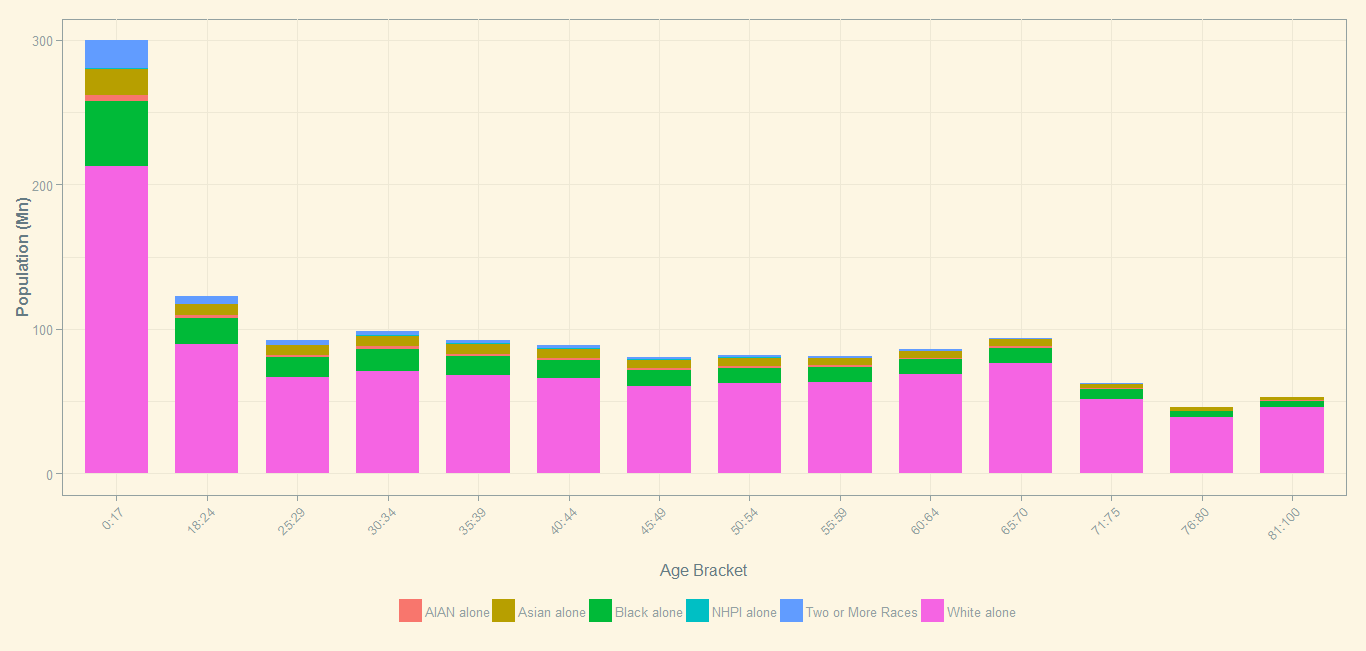
# Create the stacked bar chart
b <- ggplot(dt_year_pop_agg.m, aes(x=age_bucket, y=value/1e6, fill=code.x))
b <- b + theme_solarized() + scale_colour_solarized("blue")
b <- b + geom_bar(stat="identity", width=0.7)
b <- b + theme(axis.line.x = element_blank(), axis.title.y = element_text(face="bold",angle=90), axis.text.x = element_text(angle=45, vjust = 1, hjust=1))
b <- b + labs(x = "\nAge Bracket", y = "Population (Mn)")
b <- b + theme(legend.position = "bottom")
b <- b + theme(legend.title=element_blank()) #Reference: [Beautiful plotting in R: A ggplot2 cheatsheet | Technical Tidbits From Spatial Analysis & Data Science](http://zevross.com/blog/2014/08/04/beautiful-plotting-in-r-a-ggplot2-cheatsheet-3/#add-x-and-y-axis-labels-labs-xlab)
b